The goal of longmixr is to provide consensus clustering for longitudinal clustering performed with flexmix. It uses the approach from ConsensusClusterPlus but replaces the clustering of the longitudinal data with a flexmix model.
Installation
You can install longmixr from CRAN with:
install.packages("longmixr")You can install the latest version from github with:
remotes::install_github("cellmapslab/longmixr")If you want to render the vignette, use:
remotes::install_github("cellmapslab/longmixr", build_vignettes = TRUE, dependencies = TRUE)Please note that for the vignette a lot more dependencies are installed.
Basic usage
You need a dataset with a column that identifies the subject, a column that denotes the time point of the measurement and variables that you want to model.
set.seed(5)
test_data <- data.frame(
  patient_id = rep(1:10, each = 4),
  visit = rep(1:4, 10),
  var_1 = c(rnorm(20, -1), rnorm(20, 3)) + rep(seq(from = 0, to = 1.5, length.out = 4), 10),
  var_2 = c(rnorm(20, 0.5, 1.5), rnorm(20, -2, 0.3)) + rep(seq(from = 1.5, to = 0, length.out = 4), 10)
)
In the following approach, the variables var_1 and var_2 each are modeled as dependent on a smooth function of time, taking the multiple measurements for each subject into account. The assumption is that var_1 and var_2 represent a multivariate outcome. The modeling is specified in the flexmix drivers and the flexmix_formula:
model_list <- list(flexmix::FLXMRmgcv(as.formula("var_1 ~ .")),
                   flexmix::FLXMRmgcv(as.formula("var_2 ~ .")))
clustering <- longitudinal_consensus_cluster(
  data = test_data,
  id_column = "patient_id",
  max_k = 2,
  reps = 3,
  model_list = model_list,
  flexmix_formula = as.formula("~s(visit, k = 4) | patient_id"))
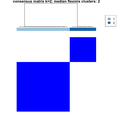
The results of the clustering can be assessed via several plots. For every specified number of clusters, the consensus matrix and the resulting hierarchical clustering on this matrix is shown. Additionally, the consensus CDF and the delta Area plots give a measure which number of cluster is optimal. The tracking plot gives an overview how the observations are distributed across the different clusters for different numbers of specified clusters. The item (subject) consensus plot shows the average consensus of each subject with all other subjects that belong to one cluster. The cluster consensus plot depicts the average consensus between all members of each cluster.
The above mentioned plots are generated when calling the plot function:
plot(clustering)You can also select which plots you want to generate:
plot(clustering, which_plots = "consensusmatrix_2")
consensus matrix plot showing two clusters cleanly separated, one bigger than the other
Detailed explanation
For a detailed explanation how you can use longmixr to analyze your longitudinal data, check out the Example clustering analysis vignette.
Cross-sectional clustering
Additionally, this package provides a wrapper function around the ConsensusClusterPlus function to work with mixed continuous and categorical data (by using the Gower distance):
dc <- mtcars
# scale continuous variables
dc <- sapply(mtcars[, 1:7], scale)
# code factor variables
dc <- cbind(as.data.frame(dc),
            vs = as.factor(mtcars$vs),
            am = as.factor(mtcars$am),
            gear = as.factor(mtcars$gear),
            carb = as.factor(mtcars$carb))
cc <- crosssectional_consensus_cluster(
  data = dc,
  reps = 10,
  seed = 1
)
Copyright
The package is based on the code of ConsensusClusterPlus (version 1.52.0). For this code the copyright holders are Matt Wilkerson and Peter Waltman. For all subsequent changes the copyright holder is the Max Planck Institute of Psychiatry. The code is licensed under GPL v2.